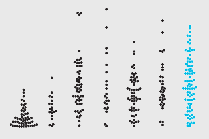
How to Make Beeswarm Plots in R to Show Distributions

Sometimes it can be beneficial to visualize the individual people, places, or things in your data rather than binning them into abstract encodings. The histogram groups data together with rectangles, and the box-and-whisker plot summarizes a dataset with quartiles. Other traditional chart types, meant to visualize distributions, do the same.

The beeswarm plot on the other hand plots all of your points in a single space. It plots the data on a single axis and then offsets in the other direction to show volume or counts.

For example, lets say you have annual incomes for 1,000 people in 2014. You could plot the data as a histogram to show the distribution of incomes. Bar height represents the number of people who made a certain annual income within an income range:

Here is the beeswarm equivalent, which represents each individual out the 1,000-person sample with a dot. The dot grouping size represents the total number of people:

It’s like a stripchart but tries to avoid overlapping dots.

In this quick R tutorial, you go over the beeswarm, making use of Aron Charles Eklund’s R package. It’s called — wait for it — beeswarm.

Setup

If you don’t have R installed yet, go ahead and do that first. It’s free, runs on the major platforms, and is typically a straightforward installation.

Assuming you have R installed, open the console and install the beeswarm package like so:

install.packages("beeswarm")

Then load it:

library("beeswarm")

That’s all you need. The rest relies on base R.

Default Beeswarm

After all, no data means no chart.On to the chart-making. Well, after you load your data with read.csv(). The data is included in the data folder in the tutorial download. Be sure to set your working directory in R to the tutorial’s folder on your computer.

# Load data
workers <- read.csv("data/income-sample-2014.tsv", sep="\t", stringsAsFactors=FALSE)

The data is a semi-random sample of 1,000 responses from the 2014 American Community Survey about total annual income. There are multiple variables, but INCTOT is the one of interest. With Eklund’s package, it’s straightforward to make a beeswarm chart with the beeswarm() function.

# Beeswarm
beeswarm(workers$INCTOT)

Here’s what you get (same chart as above):

It clutters pretty quick since it’s 1,000 points in one space, but you can categorize the incomes (INCTOT) by occupation (main_occ).

beeswarm(INCTOT ~ main_occ, data=workers, method="swarm")

You can always view the documentation by typing a question mark followed by the function name. So in the console, enter
?beeswarm.Notice the tilde (~) notation and the “swarm” method specification. The beeswarm() function also provides three other methods, which I’ll let you poke around with via the documentation.

It’s still kind of cluttered, eh? Let’s mess with more of the options to make this thing more readable.

Beeswarm Options

An explanation of the graphical parameters in base R.At this point, you can modify the beeswarm chart like you would any chart from base graphics. You can change colors (col), symbols (pch), and symbols size (cex) like so:

# Beeswarm options
beeswarm(INCTOT ~ main_occ, data=workers, col=sample(colors(), 27), pch=19, method="swarm", cex=0.5)

That’s a bit better.

If you’re interested in what the job categories actually are, you can find them on IPUMS.

But of course you can do more. MOAR! Let’s make it horizontal, change the axis labels, add a title, change the category labels, and remove the box. Because we can.

# More parameters
par(las=1)
beeswarm(INCTOT ~ main_occ, data=workers, col=sample(colors(), 27), pch=19, method="swarm", cex=0.5, horizontal=TRUE, xlab="Annual Income, Dollars", ylab="Occupation Category", main="Distribution of Income, by Occupation Caetgory", labels=c(LETTERS, "AA"), bty="n")

The result:

And that’s it. Like I said, there are more things you can fiddle with, which you can find in the documentation. Just enter ?beeswarm in the R console. You can also find more examples on Eklund’s page.

More Tutorials Worth a Look

Here are some tutorials you might also be interested in.

• Moving Past Default R Charts
• How to Visualize and Compare Distributions
• R Cheat Sheet and Guide for Graphical Parameters