When it comes to visualization, especially on the Web, you have to be open-minded, and you should be willing to try new things. There’s no advancing otherwise. However, before you dive into the advanced stuff – like just about everything in your life – you have to learn the fundamentals before you know when you can break the rules.
You have to know what flavors work together and against each other before you cook a feast fit for a king. You have to learn grammar and spelling before you can write a book that others will actually enjoy.
So when you’re learning to visualize data, do yourself a favor and learn the basic rules first. Then you can spend the rest of your days breaking them.
What Works
Luckily, researchers have already done lots of studies on what visual cues work and what sucks, so you don’t have to start from scratch. Most notable is perhaps William S. Cleveland and Robert McGill’s paper Graphical Perception: Theory, Experimentation, and Application to the Development of Graphical Methods [pdf] from the September 1984 edition of the Journal of the American Statistical Association. I won’t rehash the whole paper, but the findings of most interest here is a ranked list of how well people decode visual cues.
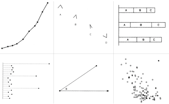
When we (the designers) visualize data, we encode the quantitative information in shapes, color, position, etc. The viewers then have to decode that information. Cleveland and McGill studied what people are able to decode most accurately and ranked them in the following list.
- Position along a common scale e.g. scatter plot
- Position on identical but nonaligned scales e.g. multiple scatter plots
- Length e.g. bar chart
- Angle & Slope (tie) e.g. pie chart
- Area e.g. bubbles
- Volume, density, and color saturation (tie) e.g. heatmap
- Color hue e.g. newsmap
I’d say that’s what we’d expect nowadays, right? However, that angle and slope ranking might be a bit of shock to some of you, given all the pie chart hate we see.
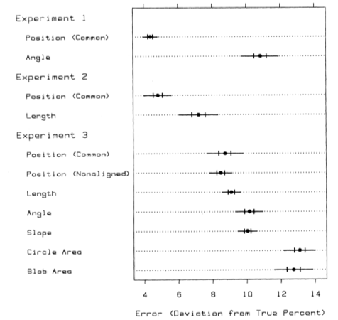
In fact, the decoding error for all encoding types isn’t wildly bad:
A Framework
Now before you go shunning everything that isn’t in the top three, keep in mind this list isn’t meant to be a definitive answer on what to use and what not to in your data graphics. Cleveland and McGill note, “The ordering does not result in a precise prescription for displaying data but rather is a framework within which to work.”
That sounds like an invitation to break some “rules” if you ask me. We might even be able to do certain things that push those error bars further left. That’s for another post though. The keyword is framework. Start with the visual fundamentals along with other important stuff, like context, the audience, and what you’re trying to accomplish, and you’ll be in good shape.
From there, you’ll learn from experience how to get fancy with your visualizations – just like how sentence fragments can be effective sometimes or how sometimes salt and fruit go well together. Sometimes area charts are a good choice.
 Visualize This: The FlowingData Guide to Design, Visualization, and Statistics (2nd Edition)
Great post, Nathan. I also found Leland Wilkinson’s “Grammar of Graphics” (http://www.amazon.com/Grammar-Graphics-Statistics-Computing/dp/0387245448/ref=sr_1_1?ie=UTF8&s=books&qid=1269145783&sr=8-1) and Colin Ware’s “Information Visualization” (http://www.amazon.com/Information-Visualization-Second-Interactive-Technologies/dp/1558608192/ref=sr_1_1?ie=UTF8&s=books&qid=1269145932&sr=1-1) very useful in this respect.
I do not think that Cleveland and McGill considered a stacked bar chart to be an example of position along nonaligned scales. On page 233 of the 1985 edition of Cleveland’s “The Elements of Graphing Data”, we see a multipanel graph with the caption saying, “Values on different panels of this graph can be compared by making judgments of positions along identical, nonaligned scales.” Figure 1 on page 532 of the paper you linked to is also suggestive of two panels. Cleveland and McGill discuss divided (or stacked) bar charts on page 533. They say:
“Figure 4 has three divided bar charts….For each of the three, the totals of A and B can be compared by perceiving the position along the scale. Position judgments can also be used to compare the two bottom positions in each case ….. All other values must be compared by the elementary task of perceiving different bar lengths”
Cleveland says “Figure 4.20 further illustrates, with made-up data, the poor performance of divided bar charts (page 261 of The Elements).
To summarize, a multipanel graph would be a better example of position along nonaligned scales while a stacked bar graph provides an example of judging lengths for all but the bottom layer and totals.
I also don’t see why a heatmap is an example of volume.
a heatmap is an example of color saturation. there are three aspects that tied there. i only provided an example for one.
right about the stacked bars. updated. thanks.
Volume is not tied with color saturation in the Cleveland and McGill paper. Volume is ranked 5 while color saturation is ranked 6. The list is slightly different in “the Elements of Graphing Data.” There, volume ranks 6 and color hue, color saturation and density tie for rank 7.
ok – so they were finicky with the rankings. i’m going off their article in Science, vol 229. that should go to show how seriously we should take the list. keyword is framework.
I did not mean to imply that their rankings were inconsistent. They are not. Rather, the ten judgments included in the rankings changed slightly. For example, color hue was included in the book but not the paper.
Very good post! The asier visualisation gets the more graphical nonsense is churned out from statistical data sources. And since it looks all so convincing it sometimes does more harm than good. Will feature this post in my Data Visualisation References resource list, aspiring to be the most comprehensive on the net. (Will be updated a little later today or tomorrow, please be patient.- Your blog is already represented in general, by the way.) If you miss anything there that I might be able to find for you or if you yourself want to share a resource, please leave a comment.
Notice that bubbles are quite far down on the list. Many of the data visualizations I’ve seen recently are based on bubbles. Some are of the same data sets that I have plotted with dot plots based on position along a common scale. There’s a world of difference in the ease of interpreting the results.
Pingback: Daily Digest for March 21st at dandube.com
Pingback: michaelgalloy.com » Fundamentals of graphical perception
Wow, the “Position along a common scale (e.g. scatter plot)” example is supposed to be EASY to decipher? I found it took quite a bit of puzzling over colors and axes before I understood what they were trying to say (and even then I didn’t really grasp the point of the chart)… isn’t a bar chart or pie chart easier to understand? (not necessarily suitable for the oxygen-vs-depth-vs-date data, just easier)
yeah, that’s not the best example. i probably should look for something more clear. the thing to remember is that basic perception was tested with basic charts. the examples provided are like the advanced counterparts.
The standard example for position along a common scale is a dot plot – see http://www.b-eye-network.com/view/2468. In fact, the dot plot was introduced by Cleveland and his colleagues at Bell Labs as a result of the experiments described in this blog post. With a scatter plot we have the position of the x coordinate against the horizontal scale and the y coordinate against the vertical scale. The example you refer to adds a third variable that is coded by color and has nothing to do with position.
You ask if a bar chart or pie chart isn’t easier to understand. Bar and pie charts are appropriate with a categorical variable and a quantitative variable while scatter plots are used with two quantitative variables, so as you pointed out, bar and pie charts are not for the data in the depth vs date data. The article in the link of the last paragraph shows advantages of the dot plot over a bar chart.
Pingback: Things I Learned This Week – #13 | dougbelshaw.com/blog
Pingback: Four short links: 8 April 2010 | Lick My Chip !
Pingback: links for 2010-04-12 « Daniel Harrison's Personal Blog
Pingback: Data & Stuff » Blog Archive » Spotted: March 25th – April 14th
Pingback: Area vs length « Mike Love’s blog
Pingback: links for 2010-06-05 « Onlinejournalismtest's Blog