Loading Data and Basic Formatting in R

Oftentimes, the bulk of the work that goes into a visualization isn’t visual at all. That is, the drawing of shapes and colors can be relatively quick, and you might spend most of your time getting the data in the format that you need (or just getting data in general).

This can be especially frustrating when you have your data, you know what you want to make, but you’re stuck in the middle. This tutorial covers the basics of getting your data into R so that you can move on to more interesting things.

Setup

Since this is in R, you need to install the free statistical computing language on your computer. Go to the R site, click on CRAN in the left sidebar (under the section titled Download, Packages), select an area near you, and download the version of R for your system. It’s a one-click install.

That’s it.

You can either use the setwd() function or you can change your working directory via the Misc > Change Working Directory… menu. You can also use absolute paths instead, but I like to save myself some typing.Now open the R console, and set your working directory to the wherever you saved the download of this tutorial to.

Loading CSV file

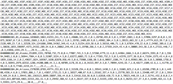
Okay, the data of this tutorial is in the data folder. It’s state-level data from the United States Census Bureau’s American Community Survey. It shows income averages for various demographics. There are several files in the folder, but the one you’re interested in is at “data/ACS_13_5YR_S1903/ACS_13_5YR_S1903.csv”. That’s the actual data file. The others are metadata.

Pass the location to the read.csv() function in R.

income <- read.csv("data/ACS_13_5YR_S1903/ACS_13_5YR_S1903.csv")

Enter dim(income) for the dimensions of the newly stored data frame.The file, with 52 rows and 123 columns, is now stored in the income variable. This loads the data with default settings, and R tries to guess what type of data you have, but sometimes it doesn’t do well. So it’s a good idea to specify some things.

For example, if you look at the second column of the actual CSV file, GEO.id2, the codes are all of length two. However, when you look at the first two columns of the data frame (income[,c(1,2)]), you can see that read.csv() removed leading zeros. That’s because R treated the column of data as numeric instead of a character. You can specify this with the colClasses argument.

# Be more specific.
income <- read.csv("data/ACS_13_5YR_S1903/ACS_13_5YR_S1903.csv", 
    stringsAsFactors=FALSE, sep=",", colClasses=c("GEO.id2"="character"))

Notice that stringsAsFactors is set to FALSE. Just do this always.

Also the separator (sep) is explicitly set to a comma to indicate that fields are comma-delimited. If you data is tab-delimited, set the value accordingly.

# Tab-delimited
income <- read.csv("data/ACS_13_5YR_S1903/ACS_13_5YR_S1903.tsv", 
    stringsAsFactors=FALSE, sep="\t", colClasses=c("GEO.id2"="character"))

If you have an internet connection, you can load data via URL. Just enter a URL where you would normally enter the directory path. The rest is the same.

# Load from URL
income <- read.csv("http://datasets.flowingdata.com/tuts/2015/load-data/ACS_13_5YR_S1903.csv", 
    stringsAsFactors=FALSE, sep=",", colClasses=c("GEO.id2"="character"))

Data at a glance

The next thing you should always do after loading data is to make sure it loaded as expected. R provides a variety of functions to look at different parts of your data.

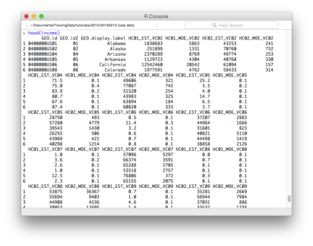
This particular dataset has 52 rows and 123 columns, so a call to head() shows quite a bit here.Enter the following to see the first handful of rows.

head(income)

The dim() function tells you the dimensions of the data frame.

dim(income)

The return value is the following, where the first value is number of rows and the second is number of columns:

[1]  52 123

Check out the column names (all 152 of them).

names(income)

And check out the structure of each column. Hopefully all is as expected. In this case, all numeric except the first two columns which are ids that indicate geographic areas.

str(income)

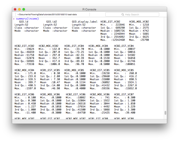
Finally, for a quick summary of each column that shows minimum, maximum, missing values, and the stuff in between, use summary().

# Quick summary
summary(income)

Subsetting

We know it’s the first seven columns because there’s a metadata file that describes each column in the data folder of the tutorial download.Maybe you just want to look at income estimates for the total population for now. This is the first seven columns (with the first two indicating region). Here’s how you subset to get a data frame with just seven columns instead of the original 153.

# Just the first columns
income_total <- income[,1:7]
head(income_total)
dim(income_total)

The new dimensions are 52 rows and 7 columns, as expected.

You can also subset based on values using subset(). Maybe you only want to look at states in the upper quartile.

# Based on value
income_upper <- subset(income_total, HC02_EST_VC02 >= 58985)

You can also remove rows with missing values in any of the fields using na.omit().

# Extract missing data (in thise case, returns empty)
income_without_na <- na.omit(income)

In this case, you get an empty data frame, because every state has at least one missing value amongst the 153 fields. In contrast, if you ran the function with income_total, you’d just get the same data frame, because no values are missing for the first seven columns.

Editing

With the data you want, it’s possible you’ll want to edit your data somehow. Maybe you want to compute new values based on existing ones, or in this case, you can rename the ambiguous columns to something more meaningful.

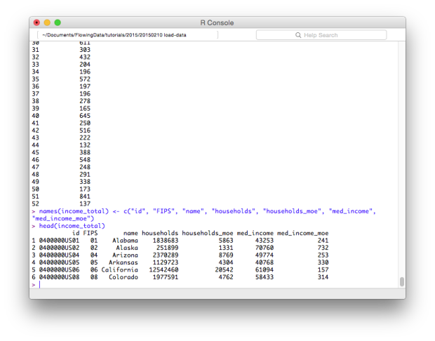
Here’s how to change column names with names(). If you just call names(), the function returns the existing column names, but if you assign it a vector of names, as shown below, you get a rename. There should be the same number of names in the vector as there are columns.

# Change column names
names(income_total) <- c("id", "FIPS", "name", "households", "households_moe", "med_income", "med_income_moe")
head(income_total)

That’s better and much easier to remember.

To access a specific column, use the dollar sign ($) after the data frame variable, followed by the name of the column. For example, if you want just the med_income column, enter income_total$med_income. Similarly, you can add columns by using the dollar sign to specify a column name and then provide a vector of values. If the column exists, the existing values are changed to the new ones and if the column name does not exist, a new column is created.

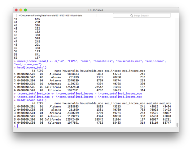
For example, in income_total, you have median and margin of error. Maybe you want to add a column for minimum and another for maximum. That’s the median income column plus and minus the margin of error.

# New columns
income_total$med_min <- income_total$med_income - income_total$med_income_moe
income_total$med_max <- income_total$med_income + income_total$med_income_moe

Want to convert units to the thousands? Divide a column by 1,000.

# Convert existing column
income_total$med_min <- income_total$med_min / 1000
income_total$med_max <- income_total$med_max / 1000

When you divide a vector by a single number, the operation is performed on each element of that vector. Same with other basic operations.

Merge with other datasets

So far you’ve loaded a single dataset, subsetted it, and added to an existing data frame. These are really common tasks you should know how to do in R. You should also know how to merge multiple datasets into one. For example, let’s say you have income data from 2008 and 2013, both for the state level.

# Load two datasets
income2008 <- read.csv("data/ACS_08_3YR_S1903/ACS_08_3YR_S1903.csv", 
    stringsAsFactors=FALSE, sep=",", colClasses=c("GEO.id2"="character"))
income2013 <- read.csv("data/ACS_13_5YR_S1903/ACS_13_5YR_S1903.csv", 
    stringsAsFactors=FALSE, sep=",", colClasses=c("GEO.id2"="character"))

And let’s just grab three columns each from 2008 and 2013: the state id, median income for the total population, and the margin of error.

# Subset
income2008p <- income2008[,c("GEO.id2", "HC02_EST_VC02", "HC02_MOE_VC02")]
income2013p <- income2013[,c("GEO.id2", "HC02_EST_VC02", "HC02_MOE_VC02")]

To make it easier to manage, give the columns names that are more useful. Remember, that these tutorials are going to mash together soon, so it’s good to use differing names for the estimate columns. For the id, which is actually a FIPS (Federal Information Processing Standards) code, we make it the same in both datasets.

# Rename headers
names(income2008p) <- c("FIPS", "med2008", "moe2008")
names(income2013p) <- c("FIPS", "med2013", "moe2013")

Here’s a glance at the two data frames before merging:

> head(income2008p)
  FIPS med2008 moe2008
1   01   42131     275
2   02   66293    1129
3   04   51124     309
4   05   39127     349
5   06   61154     173
6   08   56574     345
> head(income2013p)
  FIPS med2013 moe2013
1   01   43253     241
2   02   70760     732
3   04   49774     253
4   05   40768     330
5   06   61094     157
6   08   58433     314

Now use the merge() function to bring this together.

# Combine
income0813 <- merge(income2008p, income2013p, by="FIPS")

You can read the line above as merge income2008p and income2013p by the FIPS column and store it in income0813. Here’s the five-column data frame you get:

> head(income0813)
  FIPS med2008 moe2008 med2013 moe2013
1   01   42131     275   43253     241
2   02   66293    1129   70760     732
3   04   51124     309   49774     253
4   05   39127     349   40768     330
5   06   61154     173   61094     157
6   08   56574     345   58433     314

Save data as a file

Finally, you can save any data frame as a CSV file to use later on in a different program. Use the function write.table(). Specify the data frame, file destination, and the separator. Row names are used by default, but I typically set it to false.

write.table(income_total, "data/income-totals.csv", 
    row.names=FALSE, sep=",")

Wrapping up

To recap, you:

1. Loaded data from CSV files
2. Subsetted data frames
3. Edited data to make it easier to manage
4. Merged multiple datasets

These are basic operations in R that will give you what you need most of the time. Assuming I already have a CSV file to load, I typically don’t have to do anything more advanced than this as far as data loading and formatting is concerned.

That said, there’s still plenty more you can and will occasionally need. For example, your data might not be a delimited text file. Maybe it’s a shapefile, in which case you have to handle it differently. The xlsx package lets you load Excel files. SASxport for SAS. There are a lot of R packages.

There are also packages to help with formatting, mainly dplyr and tidyr. You can install all of them via the package installer in R.

Now you can do some visualizing.